Stratified thermal storage
Scope
This module was developed to implement a simplified model of a large-scale sensible heat storage with ideal stratification for energy system optimization with oemof.solph.
Concept
A simplified 2-zone-model of a stratified thermal energy storage.
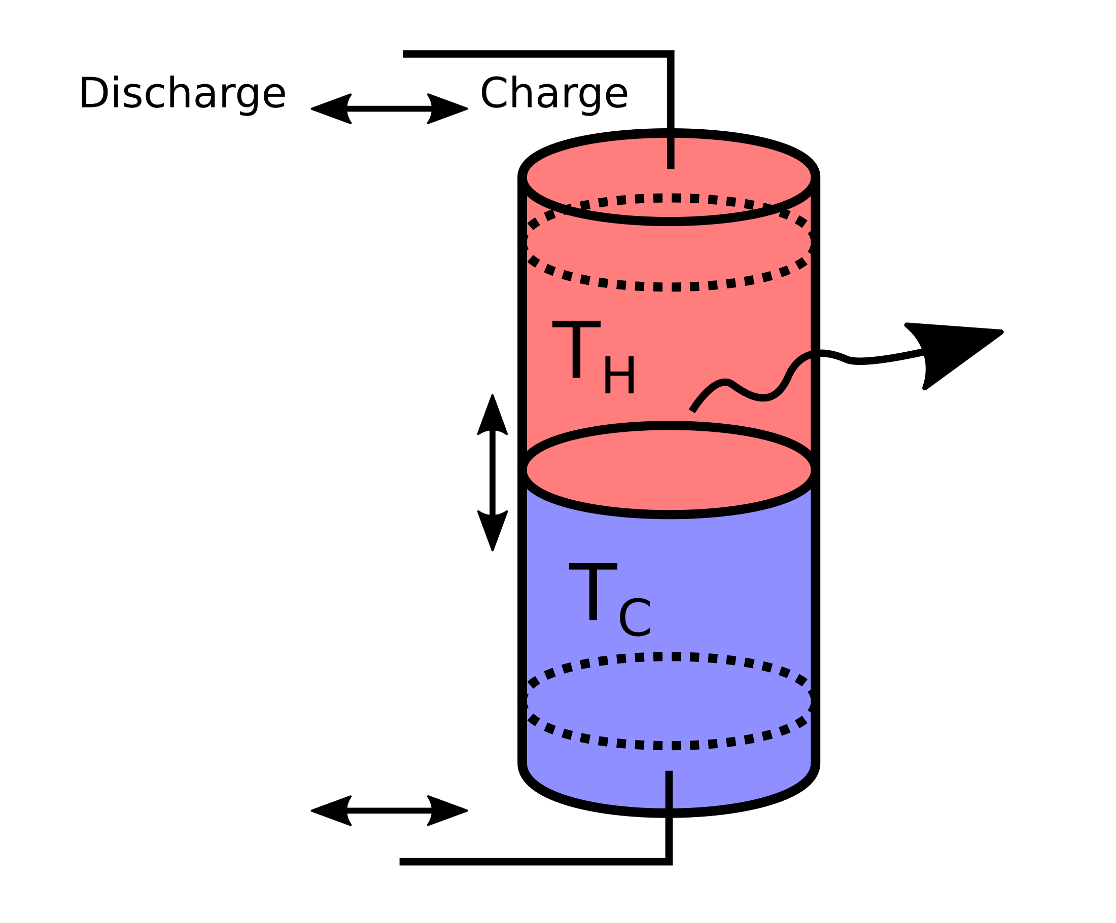
Fig. 1: Schematic of the simplified model of a stratified thermal storage with two
perfectly separated bodies of water with temperatures  and
and
 . When charging/discharging the storage, the thermocline moves
down or up, respectively. Losses to the environment through the surface of the
storage depend on the size of the hot and cold zone.
. When charging/discharging the storage, the thermocline moves
down or up, respectively. Losses to the environment through the surface of the
storage depend on the size of the hot and cold zone.
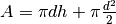
- We assume a cylindrical storage of (inner) diameter d and height h, with two temperature regions that are perfectly separated.
- The temperatures are assumed to be constant and correspond to the feed-in/return temperature of the heating system.
- Heat conductivity of the storage has to be passed as well as a timeseries of outside temperatures for the calculation of heat losses.
- There is no distinction between outside temperature and ground temperature.
- A single value for the thermal transmittance
 is assumed, neglecting the
fact that the storage’s lateral surface is bent and thus has a higher thermal
transmittance than a flat surface. The relative error introduced here gets
smaller with larger storage diameters.
is assumed, neglecting the
fact that the storage’s lateral surface is bent and thus has a higher thermal
transmittance than a flat surface. The relative error introduced here gets
smaller with larger storage diameters. - Material properties are constant.
The equation describing the storage content at timestep t is the following:

which is of the form
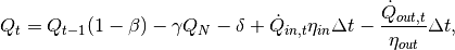
with
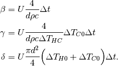
The three terms represent:
 , constant heat losses through the top and bottom surfaces,
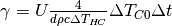
 , losses through the total lateral surface assuming the storage
to be empty (storage is at
, losses through the total lateral surface assuming the storage
to be empty (storage is at  , and
, and  is the driving
temperature difference), depending on the height of the storage,
is the driving
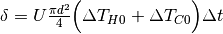
temperature difference), depending on the height of the storage, , additional losses through lateral surface that
belong to the hot part of the water body, depending on the state of charge.
, additional losses through lateral surface that
belong to the hot part of the water body, depending on the state of charge.
In the case of investment, the diameter  is given and the height can be
adapted to adapt the nominal capacity of the storage. With this assumption,
all relations stay linear.
is given and the height can be
adapted to adapt the nominal capacity of the storage. With this assumption,
all relations stay linear.
Because of the space that diffuser plates for charging/discharging take up, it is assumed that the storage can neither be fully charged nor discharged, which is parametrised as a minimal/maximal storage level (indicated by the dotted lines in Fig. 1).
These parameters are part of the stratified thermal storage module:
symbol attribute type explanation heightHeight [m] (if not investment) diameterDiameter [m] surfaceStorage surface [m2] volumeStorage volume [m3] densityDensity of storage medium [kg/m3] heat_capacityHeat capacity of storage medium [J/(kg*K)] temp_hHot temperature level [deg C] temp_cCold temperature level [deg C] temp_envEnvironment temperature timeseries [deg C] attribute of oemof-solph component Stored thermal energy at time t [MWh] attribute of oemof-solph component Energy flowing in at time t nominal_storage_capacityMaximum amount of stored thermal energy [MWh] u_valueThermal transmittance [W/(m2*K)] s_isoThickness of isolation layer [mm] lamb_isoHeat conductivity of isolation material [W/(m*K)] alpha_insideHeat transfer coefficient inside [W/(m2*K)] alpha_outsideHeat transfer coefficient outside [W/(m2*K)] loss_rateRelative loss of storage content within one timestep [-] fixed_losses_relativeFixed losses as share of nominal storage capacity [-] fixed_losses_absoluteFixed absolute losses independent of storage content or nominal storage capacity [MWh] inflow_conversion_factorCharging efficiency [-] outflow_conversion_factorDischarging efficiency [-]


Usage
StratifiedThermalStorage facade
Using the StratifiedThermalStorage facade, you can instantiate a storage like this:
from oemof.solph import Bus
from oemof.thermal.facades import StratifiedThermalStorage

bus_heat = Bus('heat')

thermal_storage = StratifiedThermalStorage(
    label='thermal_storage',
    bus=bus_heat,
    diameter=2,
    height=5,
    temp_h=95,
    temp_c=60,
    temp_env=10,
    u_value=u_value,
    min_storage_level=0.05,
    max_storage_level=0.95,
    capacity=1,
    efficiency=0.9,
    marginal_cost=0.0001
)
The non-usable storage volume is represented by the parameters
min_storage_level and max_storage_level.
To learn about all parameters that can be passed to the facades, have a look at the API documentation of the StratifiedThermalStorage class of the facade module.
For the storage investment mode, you still need to provide diameter, but
leave height and capacity open and set expandable=True.
There are two options to choose from:
- Invest into
nominal_storage_capacityandcapacity(charging/discharging power) with a fixed ratio. Passinvest_relation_input_capacityand eitherstorage_capacity_costorcapacity_cost. - Invest into
nominal_storage_capacityandcapacityindependently with no fixed ratio. Passstorage_capacity_costandcapacity_cost.
In many practical cases, thermal storages are dimensioned using a rule of thumb: The storage should be able to provide its peak thermal power for 6-7 hours. To apply this in a model, use option 1.
thermal_storage = StratifiedThermalStorage(
    label='thermal_storage',
    bus=bus_heat,
    diameter=2,
    temp_h=95,
    temp_c=60,
    temp_env=10,
    u_value=u_value,
    expandable=True,
    capacity_cost=0,
    storage_capacity_cost=400,
    minimum_storage_capacity=1,
    invest_relation_input_capacity=1 / 6,
    min_storage_level=0.05,
    max_storage_level=0.95,
    efficiency=0.9,
    marginal_cost=0.0001
)
If you do not want to use a rule of thumb and rather let the model decide, go with option 2. Do so
by leaving out invest_relation_input_capacity and setting capacity_cost to
a finite value. Also have a look at the examples, where both options are shown.
A 3rd and 4th option, investing into nominal_storage_capacity but leaving
capacity fixed or vice versa, can not be modelled with this facade (at the moment).
It seems to be a case that is not as relevant for thermal storages as the others. If you want to
model it, you can do so by performing the necessary pre-calculations and using oemof.solph’s
GenericStorage directly.
Warning
For this example to work as intended, please use oemof-solph v0.4.0 or higher
to ensure that the GenericStorage has the attributes fixed_losses_absolute and
fixed_losses_relative.
The following figure shows a comparison of results of a common storage implementation using only a loss rate vs. the stratified thermal storage implementation (source code).
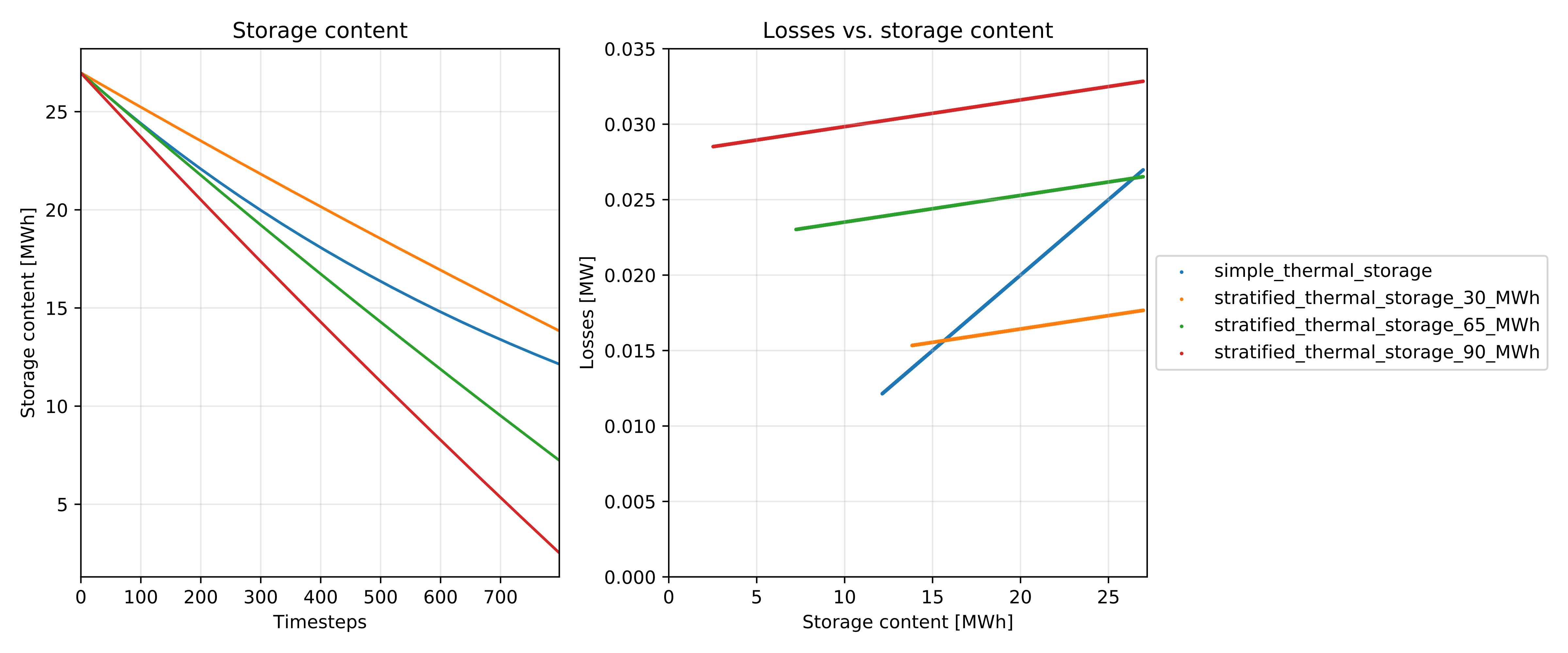
Fig. 2: Example plot showing the difference between StratifiedThermalStorages
of different storage capacities and a simpler model with a single loss rate. The left panel
shows the loss of thermal energy over time. The right panel shows losses vs. storage content.
Implicit calculations
In the background, the StratifiedThermalStorage class uses the following functions. They can be used independent of the facade class as well.
The thermal transmittance is pre-calculated using calculate_u_value.
The dimensions of the storage are calculated with calculate_storage_dimensions
volume, surface = calculate_storage_dimensions(height, diameter)

The nominal storage capacity is pre-calculated using calculate_capacities.
nominal_storage_capacity = calculate_capacities(
    volume, temp_h, temp_c, heat_capacity, density
)

Loss terms are precalculated by the following function.
loss_rate, fixed_losses_relative, fixed_losses_absolute = calculate_losses(
    u_value, diameter, temp_h, temp_c, temp_env,
    time_increment, heat_capacity, density)

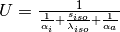
To calculate the thermal transmittance of the storage hull from material properties, you can use the following function.
u_value = calculate_storage_u_value(s_iso, lamb_iso, alpha_inside, alpha_outside)