Concentrating solar power
Module to calculate the usable heat of a parabolic trough collector
Scope
This module was developed to provide the heat of a parabolic trough collector based on temperatures and collectors location, tilt and azimuth for energy system optimizations with oemof.solph.
In https://github.com/oemof/oemof-thermal/tree/dev/examples you can find an example on how to use the modul to calculate a CSP power plant. A time series of pre-calculated heat flows can be used as input for a source (an oemof.solph component), and a transformer (an oemof.solph component) can be used to hold electrical power consumption and further thermal losses of the collector in an energy system optimization. In addition, you will find an example which compares this precalculation with a calculation using a constant efficiency.
Concept
The pre-calculations for the concentrating solar power calculate the heat of the solar collector based on the direct horizontal irradiance (DHI) or the direct normal irradiance (DNI) and information about the collector and its location. The losses can be calculated in 2 different ways.
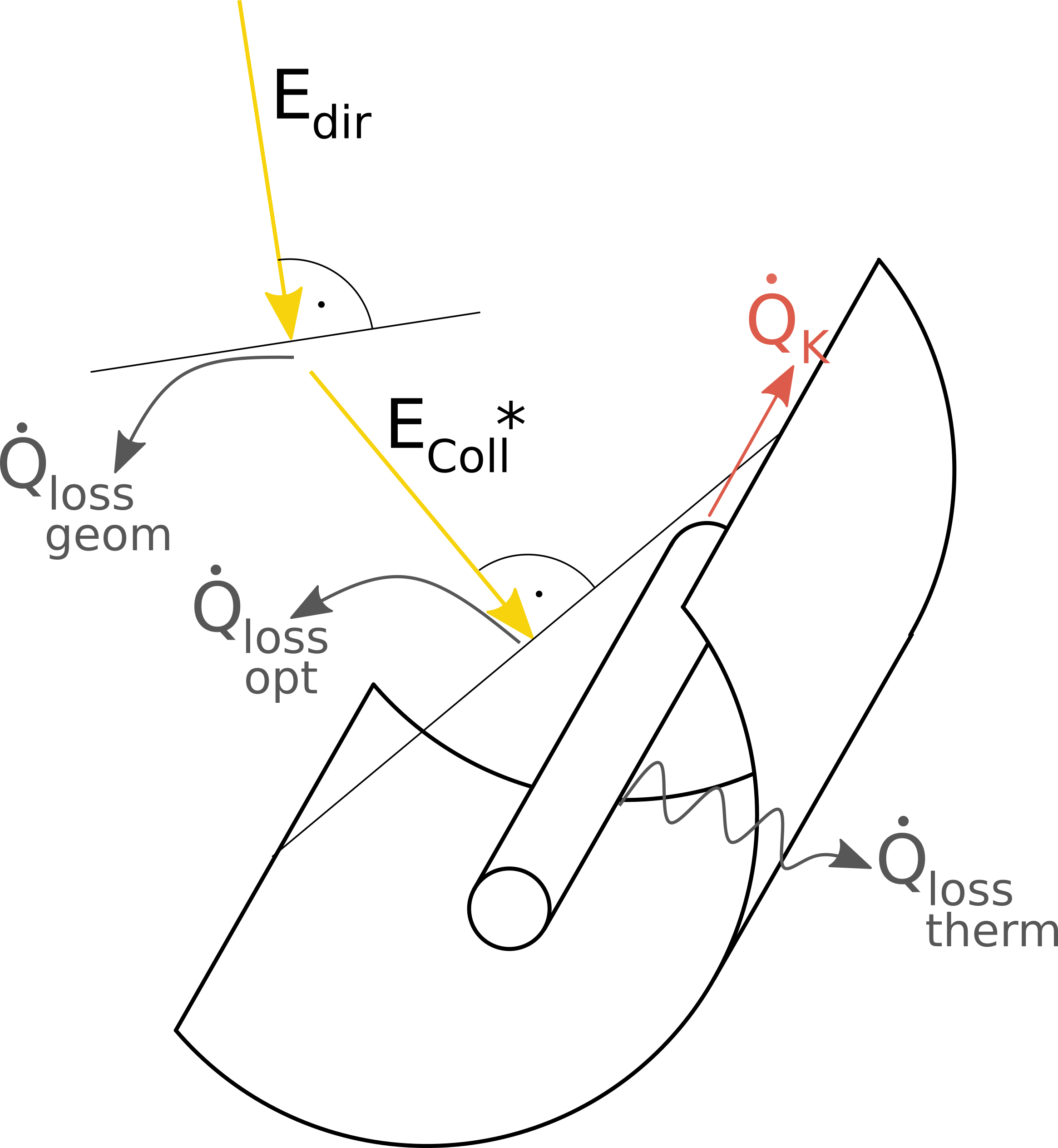
Fig.1: The energy flows and losses at a parabolic trough collector.
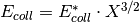
The direct normal radiation ( ) is reduced by geometrical losses
(
) is reduced by geometrical losses
( ) so that only the collector radiation
(
) so that only the collector radiation
( ) hits the collector. Before the thermal power is absorbed by
the absorber tube, also optical losses (
) hits the collector. Before the thermal power is absorbed by
the absorber tube, also optical losses ( ), which can
be reflection losses at the mirror, transmission losses at the cladding tube
and absorption losses at the absorber tube, occur. The absorber finally loses a
part of the absorbed heat output through thermal losses
(
), which can
be reflection losses at the mirror, transmission losses at the cladding tube
and absorption losses at the absorber tube, occur. The absorber finally loses a
part of the absorbed heat output through thermal losses
( ).
).
The processing of the irradiance data is done by the pvlib, which calculates the direct irradiance on the collector. This irradiance is reduced by dust and dirt on the collector with:
The efficiency of the collector is calculated depending on the loss method with
method ‘Janotte’:
method ‘Andasol’:

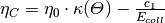
with the incident angle modifier, which is calculated depending on the loss method:
method ‘Janotte’:
method ‘Andasol’:


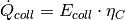
In the end, the irradiance on the collector is multiplied with the efficiency to get the collector’s heat.
The three values  ,
,  and
and  are
returned. Losses which occur after the heat absorption in the collector
(e.g. losses in pipes) have to be taken into account in a later step
(see the example).
are
returned. Losses which occur after the heat absorption in the collector
(e.g. losses in pipes) have to be taken into account in a later step
(see the example).
These arguments are used in the formulas of the function:
symbol argument explanation collector_irradianceIrradiance on collector considering all losses including losses because of dirtiness irradiance_on_collectorIrradiance which hits collectors surface before losses because of dirtiness are considered cleanlinessCleanliness of the collector (between 0 and 1) iamIncidence angle modifier a_1Parameter 1 for the incident angle modifier a_2Parameter 2 for the incident angle modifier a_3Parameter 3 for the incident angle modifier a_4Parameter 4 for the incident angle modifier a_5Parameter 5 for the incident angle modifier a_6Parameter 6 for the incident angle modifier aoiAngle of incidence eta_cCollector efficiency c_1Thermal loss parameter 1 c_2Thermal loss parameter 2 delta_tTemperature difference (collector to ambience) eta_0Optical efficiency of the collector collector_heatCollector’s heat


Usage
It is possible to use the precalculation function as stand-alone function to
calculate the collector values , and
. Or it is possible to use the ParabolicTroughCollector facade
to model a collector with further losses (e.g. in pipes or pumps) and the
electrical consumption of pipes within a single step.
Please note: As the unit of the input irradiance is given as power per area,
the outputs and are given in the same
unit. If these values are used in an oemof source, the unit of the nominal
value must be an area too.
Precalculation function
Please see the API documentation of the concentrating_solar_power
module for all parameters which have to be provided, also the ones that are
not part of the described formulas above.
The data for ambient temperature and irradiance must have the same time index.
Depending on the method, the irradiance must be the horizontal direct
irradiance or the direct normal irradiance. Be aware of the correct time index
regarding the time zone, as the utilized pvlib need the correct time stamp
corresponding to the location (latitude and longitude).
data_precalc = csp_precalc(
    latitude, longitude,
    collector_tilt, collector_azimuth, cleanliness,
    eta_0, c_1, c_2,
    temp_collector_inlet, temp_collector_outlet, dataframe['t_amb'],
    a_1, a_2,
    E_dir_hor=dataframe['E_dir_hor']
    )
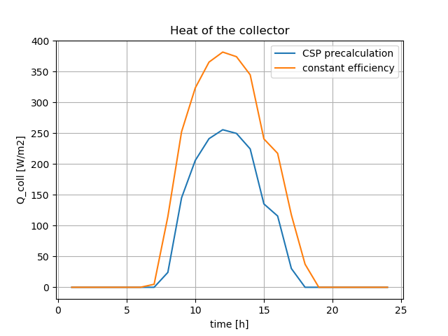
The following figure shows the heat provided by the collector calculated with this functions and the loss method “Janotte” in comparison to the heat calculated with a fix efficiency.
The results of this precalculation can be used in an oemof energy system model as output of a source component. To model the behaviour of a collector, it can be complemented with a transformer, which holds the electrical consumption of pumps and peripheral heat losses (see the the example csp_plant_collector.py).
ParabolicTroughCollector facade
Instead of using the precalculation, it is possible to use the
ParabolicTroughCollector facade, which will create an oemof component as a
representative for the collector. It calculates the heat of the collector in
the same way as the precalculation do. Additionally, it integrates the
calculated heat as an input into a component, uses an electrical input for
pumps and gives a heat output, which is reduced by the defined additional losses.
As given in the example, further parameters are required in addition to the
ones of the precalculation. Please see the API documentation of the ParabolicTroughCollector
class of the facade module for all parameters which have to be provided.
See example_csp_facade.py for an application example. It models the same system as the csp_plant_example.py, but uses the ParabolicTroughCollector facade instead of separate source and transformer.
from oemof import solph
    >>> from oemof.thermal.facades import ParabolicTroughCollector
    >>> bth = solph.Bus(label='thermal_bus')
    >>> bel = solph.Bus(label='electrical_bus')
    >>> collector = ParabolicTroughCollector(
    ...     label='solar_collector',
    ...     heat_bus=bth,
    ...     electrical_bus=bel,
    ...     electrical_consumption=0.05,
    ...     additional_losses=0.2,
    ...     aperture_area=1000,
    ...     loss_method='Janotte',
    ...     irradiance_method='horizontal',
    ...     latitude=23.614328,
    ...     longitude=58.545284,
    ...     collector_tilt=10,
    ...     collector_azimuth=180,
    ...     x=0.9,
    ...     a_1=-0.00159,
    ...     a_2=0.0000977,
    ...     eta_0=0.816,
    ...     c_1=0.0622,
    ...     c_2=0.00023,
    ...     temp_collector_inlet=435,
    ...     temp_collector_outlet=500,
    ...     temp_amb=input_data['t_amb'],
    ...     irradiance=input_data['E_dir_hor']
    )
References
[1] Janotte, N; et al: Dynamic performance evaluation of the HelioTrough collector demon-stration loop - towards a new benchmark in parabolic trough qualification, SolarPACES 2013
[2] William F. Holmgren, Clifford W. Hansen, and Mark A. Mikofski. “pvlib python: a python package for modeling solar energy systems.” Journal of Open Source Software, 3(29), 884, (2018). https://doi.org/10.21105/joss.00884