Solar thermal collector¶

Module to calculate the usable heat of a flat plate collector.

Scope¶

This module was developed to provide the heat of a flat plate collector based on temperatures and collector’s location, tilt and azimuth for energy systems optimizations with oemof.solph.

In https://github.com/oemof/oemof-thermal/tree/dev/examples you can find an example, how to use the modul to calculate a system with flat plate collector, storage and backup to provide a given heat demand. The time series of the pre-calculated heat is output of a source (an oemof.solph component) representing the collector, and a transformer (an oemof.solph component) is used to hold electrical power consumption and further thermal losses of the collector in an energy system optimization. In addition, you will find a plot, which compares this precalculation with a calculation with a constant efficiency.

Concept¶

The precalculations for the solar thermal collector calculate the heat of the solar collector based on global and diffuse horizontal irradiance and information about the collector and the location. The following scheme shows the calculation procedure.

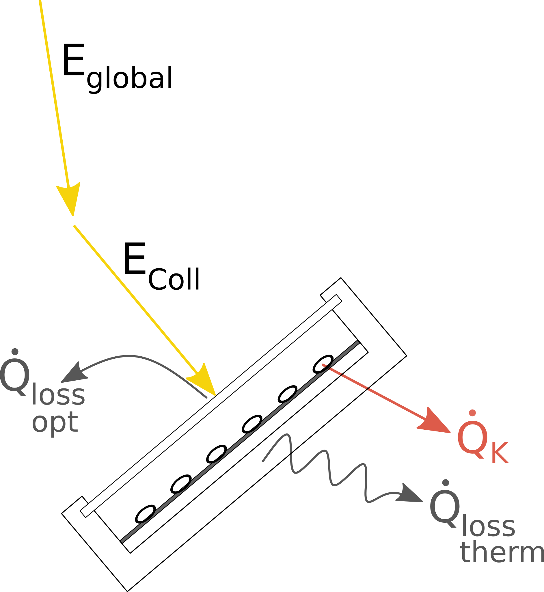
Fig.1: The energy flows and losses at a flat plate collector.

The processing of the irradiance data is done by the pvlib, which calculates the total in-plane irradiance according to the azimuth and tilt angle of the collector.

The efficiency of the collector is calculated with

$\eta_C = \eta_0 - a_1 \cdot \frac{\Delta T}{E_{coll}} - a_2 \cdot \frac{{\Delta T}^2}{E_{coll}}$

with

$\Delta T = T_{coll,in} + {\Delta T}_n - T_{amb}$

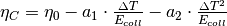
In the end, the irradiance on the collector is multiplied with the efficiency to get the collectors heat.

$\dot Q_{coll} = E_{coll} \cdot \eta_C$

The three values $\dot Q_{coll}$ , $\eta_C$ and $E_{coll}$ are returned in a dataframe. Losses, which occur after the heat absorption in the collector (e.g. losses in pipes) have to be taken into account in the component, which uses the precalculation (see the example).

These arguments are used in the formulas of the function:

symbol argument explanation

$E_{coll}$ collector_irradiance Irradiance on collector after all losses

$\eta_C$ eta_c Collectors efficiency

$a_1$ a_1 Thermal loss parameter 1

$a_2$ a_2 Thermal loss parameter 2

$\Delta T$ delta_t Temperature difference (collector to ambience)

$T_{coll, in}$ temp_collector_inlet Collectors inlet temperature

$\Delta T_n$ delta_temp_n Temperature difference between collector inlet and mean temperature

$T_{amb}$ temp_amb Ambient temperature

$\eta_0$ eta_0 Optical efficiency of the collector

$\dot Q_{coll}$ collector_heat Collectors heat

Usage¶

It is possible to use the precalculation function as stand-alone function to calculate the collector values $\dot Q_{coll}$ , $\eta_C$ and $E_{coll}$ . Or it is possible to use the SolarThermalCollector facade to model a collector with further losses (e.g. in pipes or pumps) and the electrical consumption of pipes within a single step. Please note: As the unit of the input irradiance is given as power per area, the outputs $\dot Q_{coll}$ and $E_{coll}$ are given in the same unit. If these values are used in an oemof source, the unit of the nominal value must be an area too.

Solar thermal collector precalculations¶

Please see the API documentation of the solar_thermal_collector module for all parameters which have to be provided, also the ones that are not part of the described formulas above. The data for the irradiance and the ambient temperature must have the same time index. Be aware of the correct time index regarding the time zone, as the utilized pvlib needs the correct time stamp corresponding to the location.

precalc_data = flat_plate_precalc(
    latitude,
    longitude,
    collector_tilt,
    collector_azimuth,
    eta_0,
    a_1,
    a_2,
    temp_collector_inlet,
    delta_temp_n,
    irradiance_global=input_data['global_horizontal_W_m2'],
    irradiance_diffuse=input_data['diffuse_horizontal_W_m2'],
    temp_amb=input_data['temp_amb'],
)

The input_data must hold columns for the global and diffuse horizontal irradiance and the ambient temperature.

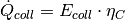
The following figure shows the heat provided by the collector calculated with this function in comparison to the heat calculated with a fix efficiency.

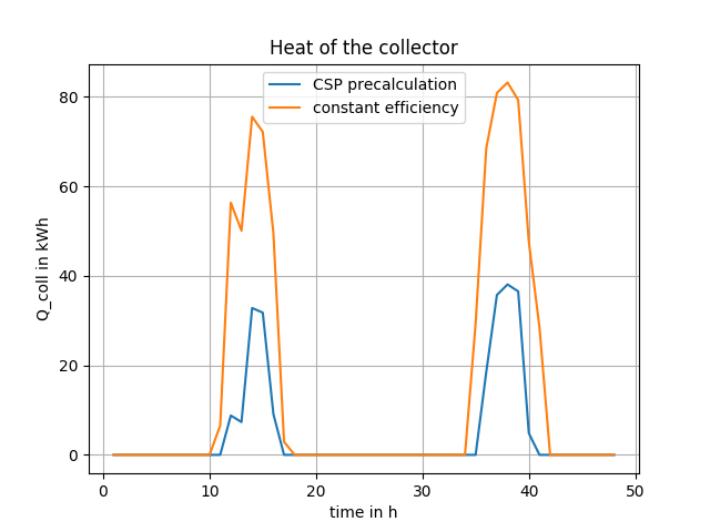
The results of this precalculation can be used in an oemof energy system model as output of a source component. To model the behaviour of a collector, it can be complemented with a transformer, which holds the electrical consumption of pumps and peripheral heat losses (see the the examples flat_plate_collector_example.py and flat_plate_collector_example_investment.py).

SolarThermalCollector facade¶

Instead of using the precalculation, it is possible to use the SolarThermalCollector facade, which will create an oemof component as a representative for the collector. It calculates the heat of the collector in the same way as the precalculation do. Additionally, it integrates the calculated heat as an input into a component, uses an electrical input for pumps and gives a heat output, which is reduced by the defined additional losses. As given in the example, further parameters are required in addition to the ones of the precalculation. Please see the API documentation of the SolarThermalCollector class of the facade module for all parameters which have to be provided.

See flat_plate_collector_example_facade.py for an application example. It models the same system as the flat_plate_collector_example.py, but uses the SolarThermalCollector facade instead of separate source and transformer.

from oemof import solph
from oemof.thermal.facades import SolarThermalCollector
bth = solph.Bus(label='thermal')
bel = solph.Bus(label='electricity')
collector = SolarThermalCollector(
    label='solar_collector',
    heat_out_bus=bth,
    electricity_in_bus=bel,
    electrical_consumption=0.02,
    peripheral_losses=0.05,
    aperture_area=1000,
    latitude=52.2443,
    longitude=10.5594,
    collector_tilt=10,
    collector_azimuth=20,
    eta_0=0.73,
    a_1=1.7,
    a_2=0.016,
    temp_collector_inlet=20,
    delta_temp_n=10,
    irradiance_global=input_data['global_horizontal_W_m2'],
    irradiance_diffuse=input_data['diffuse_horizontal_W_m2'],
    temp_amb_col=input_data['temp_amb'],
)