Absorption chiller¶

Calculations for absorption chillers based on the characteristic equation method.

Scope¶

This module was developed to provide cooling capacity and COP calculations based on temperatures for energy system optimizations with oemof.solph.

Concept¶

A characteristic equation model to describe the performance of absorption chillers.

Fig.1: Absorption cooling (or heating) process.

The cooling capacity ( $\dot{Q}_{E}$ ) is determined by a function of the characteristic temperature difference ( $\Delta\Delta t'$ ) that combines the external mean temperatures of the heat exchangers.

Various approaches of the characteristic equation method exists. Here we use the approach described by Kühn and Ziegler [1]:

$\Delta\Delta t' = t_{G} - a \cdot t_{AC} + e \cdot t_{E}$

with the assumption

$t_{A} = t_{C} = t_{AC}$

where $t$ is the external mean fluid temperature of the heat exchangers (G: Generator, AC: Absorber and Condenser, E: Evaporator) and $a$ and $e$ are characteristic parameters.

The cooling capacity ( $\dot{Q}_{E}$ ) and the driving heat ( $\dot{Q}_{G}$ ) can be expressed as linear functions of $\Delta\Delta t'$ :

$\dot{Q}_{E} = s_{E} \cdot \Delta\Delta t' + r_{E}$

$\dot{Q}_{G} = s_{G} \cdot \Delta\Delta t' + r_{G}$

with the characteristic parameters $s_{E}$ , $r_{E}$ , $s_{G}$ , and $r_{G}$ .

The COP can then be calculated from $\dot{Q}_{E}$ and $\dot{Q}_{G}$ :

$COP = \frac{\dot{Q}_{E}}{\dot{Q}_{G}}$

These arguments are used in the formulas of the function:

symbol argument explanation

$\Delta\Delta t'$ ddt Characteristic temperature difference

$t_G$ t_hot External mean fluid temperature of generator

$t_{AC}$ t_cool External mean fluid temperature of absorber and condenser

$t_E$ t_chill External mean fluid temperature of evaporator

$a$ coef_a Characteristic parameter

$e$ coef_e Characteristic parameter

$s$ coef_s Characteristic parameter

$r$ coef_r Characteristic parameter

$\dot{Q}$ Q_dots Heat flux

$\dot{Q}_{E}$ Q_dots_evap Cooling capacity (heat flux at evaporator)

$\dot{Q}_{G}$ Q_dots_gen Driving heat (heat flux at generator)

$COP$ COP Coefficient of performance

Usage¶

The following example shows how to calculate the COP of a small absorption chiller. The characteristic coefficients used in this examples belong to a 10 kW absorption chiller developed and tested at the Technische Universität Berlin [1].

import oemof.thermal.absorption_heatpumps_and_chillers as abs_chiller

# Characteristic temperature difference
ddt = abs_chiller.calc_characteristic_temp(
    t_hot=[85],  # in °C
    t_cool=[26],  # in °C
    t_chill=[15],  # in °C
    coef_a=10,
    coef_e=2.5,
    method='kuehn_and_ziegler')

# Cooling capacity
Q_dots_evap = abs_chiller.calc_heat_flux(
    ddts=ddt,
    coef_s=0.42,
    coef_r=0.9,
    method='kuehn_and_ziegler')

# Driving heat
Q_dots_gen = abs_chiller.calc_heat_flux(
    ddts=ddt,
    coef_s=0.51,
    coef_r=2,
    method='kuehn_and_ziegler')

COPs = Q_dots_evap / Q_dots_gen

Fig.2 illustrates how the cooling capacity and the COP of an absorption chiller (here the 10 kW absorption chiller mentioned above) depend on the cooling water temperature, i.e. the mean external fluid temperature at absorber and condenser.

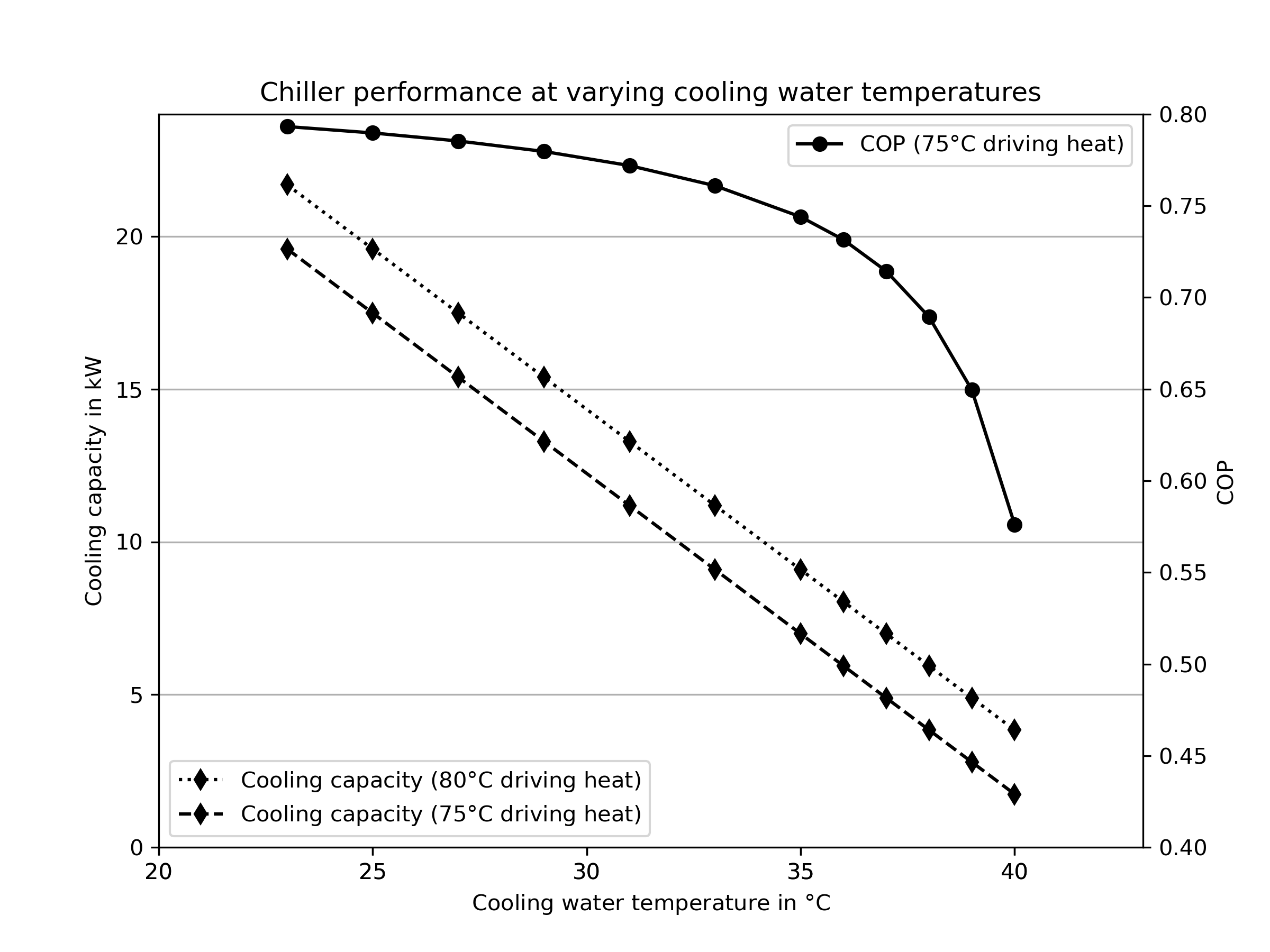
cooling_capacity_over_cooling_water_temperature_Kuehn.png

Fig.2: Dependency of the cooling capacity and the COP of a 10 kW absorption chiller on the cooling water temperature.

You find the code that is behind Fig.2 in our examples: https://github.com/oemof/oemof-thermal/tree/master/examples

You can run the calculations for any other absorption heat pump or chiller by entering the specific parameters (a, e, s, r) belonging to that specific machine. The specific parameters are determined by a numerical fit of the four parameters with testing data or data from the fact sheet (technical specifications from the manufacturer) if temperatures for at least two points of operation are given. You find detailed information in the referenced papers.

This package comes with characteristic parameters for five absorption chillers. Four published by Puig-Arnavat et al. [3]: ‘Rotartica’, ‘Safarik’, ‘Broad_01’ and ‘Broad_02’ and one published by Kühn and Ziegler [1]: ‘Kuehn’. If you like to contribute parameters for other machines, please feel free to contact us or to contribute directly via github.

To model one of the machines provided by this package you can adapt the code above in the following way.

import oemof.thermal.absorption_heatpumps_and_chillers as abs_chiller
import pandas as pd
import os

filename_charpara = os.path.join(os.path.dirname(__file__), 'data/characteristic_parameters.csv')
charpara = pd.read_csv(filename_charpara)

chiller_name = 'Kuehn'  # 'Rotartica', 'Safarik', 'Broad_01', 'Broad_02'

 # Characteristic temperature difference
ddt = abs_chiller.calc_characteristic_temp(
    t_hot=[85],  # in °C
    t_cool=[26],  # in °C
    t_chill=[15],  # in °C
    coef_a=charpara[(charpara['name'] == chiller_name)]['a'].values[0],
    coef_e=charpara[(charpara['name'] == chiller_name)]['e'].values[0],
    method='kuehn_and_ziegler')

# Cooling capacity
Q_dots_evap = abs_chiller.calc_heat_flux(
    ddts=ddt,
    coef_s=charpara[(charpara['name'] == chiller_name)]['s_E'].values[0],
    coef_r=charpara[(charpara['name'] == chiller_name)]['r_E'].values[0],
    method='kuehn_and_ziegler')

# Driving heat
Q_dots_gen = abs_chiller.calc_heat_flux(
    ddts=ddt,
    coef_s=charpara[(charpara['name'] == chiller_name)]['s_G'].values[0],
    coef_r=charpara[(charpara['name'] == chiller_name)]['r_G'].values[0],
    method='kuehn_and_ziegler')

COPs = [Qevap / Qgen for Qgen, Qevap in zip(Q_dots_gen, Q_dots_evap)]

You find information on the machines in [1], [2] and [3]. Please be aware that [2] introduces a slightly different approach (using an improved characteristic equation with $\Delta\Delta t''$ instead of $\Delta\Delta t'$ ). The characteristic parameters that we use are derived from [1] and therefore differ from those in [2].

References¶

[1] A. Kühn, F. Ziegler. “Operational results of a 10 kW absorption chiller and adaptation of the characteristic equation”, Proc. of the 1st Int. Conf. Solar Air Conditioning, 6-7 October 2005, Bad Staffelstein, Germany.

[2] A. Kühn, C. Özgür-Popanda, and F. Ziegler. “A 10 kW indirectly fired absorption heat pump : Concepts for a reversible operation,” in Thermally driven heat pumps for heating and cooling, Universitätsverlag der TU Berlin, 2013, pp. 173–184. [http://dx.doi.org/10.14279/depositonce-4872]

[3] Maria Puig-Arnavat, Jesús López-Villada, Joan Carles Bruno, Alberto Coronas. Analysis and parameter identification for characteristic equations of single- and double-effect absorption chillers by means of multivariable regression. In: International Journal of Refrigeration, 33 (2010) 70-78.